The Singular Value Perspective
A deep dive on the singular value decomposition, a powerful tool for understanding and visualizing matrices.
If you already have a good grasp of SVD, feel free to skim the first few sections.
Introduction
Matrices are everywhere in Machine Learning. They are the fundamental unit of computation. To maximally contribute to a field, it would be wise to intimately understand the fundamental units of that field.
Still, matrices can feel unintuitive and confusing for many of us. A few common (yet poorly undersood) topics include:
1. Shearings of space
2. Transposes and Rectangular matrices
3. Inverses and psuedoinverses
4. Principal Component Analysis
These topics don’t have to feel so opaque. After setting out to deeply understand this unit of computation, ubiquitious across all architectures, this post represents a culmination of learning. The perspectives gained, which are being shared for the first time in this post, have greatly increased my productivity as an ML researcher.
2. I have a far stronger understanding of computation capabilities in transformers (future post).
3. I doubled the performance boost of a complex embedding technique within 90 days of joining that ML subfield.
In short, I took the time to write this post because I have seen firsthand that deeply understanding this topic has been quite valuable for me, and I hope more people can benefit from it too!
Before we dive in, we should clarify that despite the length of this post, your takeaway will be surprisingly straightforward. You won’t be overwhelmed by the complexity of the Singular Value Decomposition (SVD); in fact, it’s likely you’ll find it simple and intuitive. Still, it’s great for the reader to have a complete document that motivates the concept and provides many examples to learn from.
Now, we will strive to master the SVD, which is essential for intuiting key concepts in linear algebra and machine learning.
An Analogy: “Track the Point”
- Sir Isaac Newton
To motivate our exploration, let’s begin with an analogy for how many of us are thinking about matrices before our SVD enlightenement.
Imagine a teacher wants us to keep track of how a 2d point changes over time. The teacher will first touch the starting location on a sheet of paper, and then we will need to keep track of where it goes next by writing down its coordinates. The teacher will say simple instructions, like “move it right [this much]” or “move it up [this much]”.
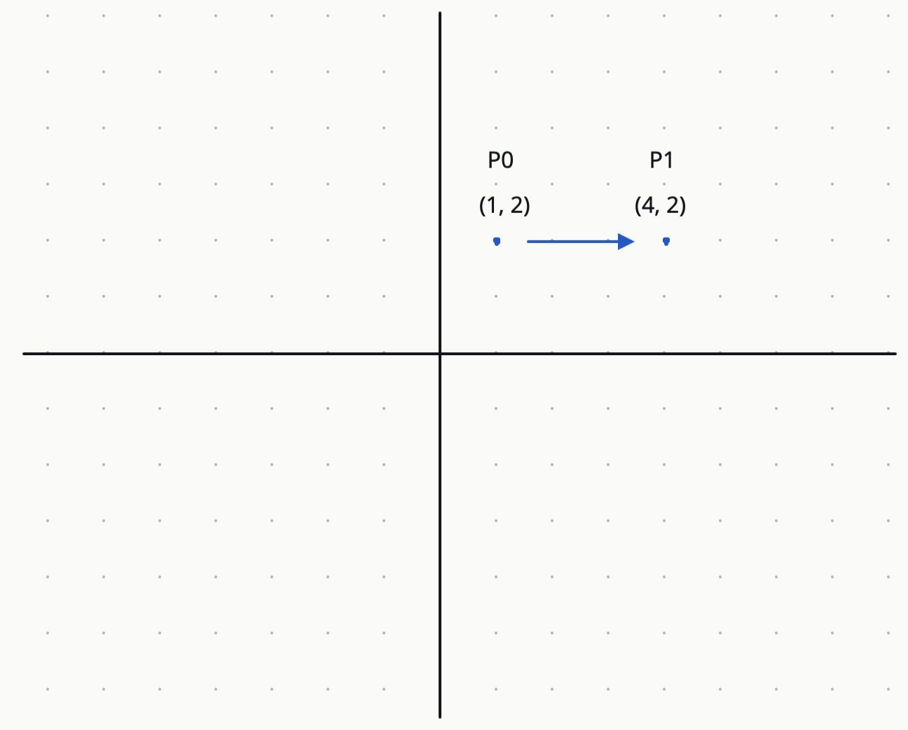
Then the teacher says "move it right 3" so we end up with the new coordinate being (4,2).
Not too hard right? Even middle schoolers could do this. But what if the coordinate axes we drew to track our point looked like this:
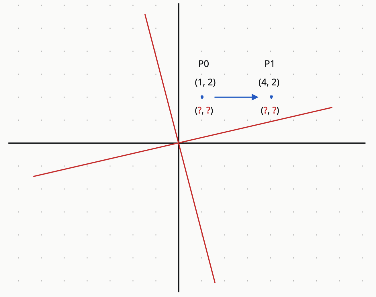
Now the task won’t only take 100 times as long, but it will be very tiring! Any time one direction is changed (e.g. “move right 3”) we have to think about how it affects all the directions and do lots of computations. Wouldn’t it be beautiful if we could understand how one dimension would change without having to think about the other ones?
The same applies to matrices: once we pick the right basis, understanding how vectors are transformed becomes much simpler. To summarize the rest of this post in one sentence: once you pick the right basis, understanding a matrix in \(n\) dimensions is basically as hard as understanding this “Track the Point” problem in \(n\) dimensions.
Defining Matrices
Let’s start by defining a matrix, and then we’ll talk about the lens through which we think about matrix transformations.
Formal Definition
A matrix \(A \in R^{m \times n}\) transforms a vector \(\vec{x} \in R^{n}\) to a vector \(A\vec{x} \in R^m\). \(A\) consists of \(n\) column vectors \(\vec{a_1}\), \(\vec{a_2}\), …, \(\vec{a_n} \in \mathbb{R}^m\) .
\[A = \begin{bmatrix} \\ \vec{a_1} & \vec{a_2} & \dots & \vec{a_n} \\ \\ \end{bmatrix}\]To multiply a matrix \(A\) by a vector \(x\), we first write \(x\) as a sum of basis vectors:
\[\begin{align*} \vec{x} = \begin{bmatrix} x_1 \\ x_2 \\ \vdots \\ x_n \\ \end{bmatrix} &= x_1 \begin{bmatrix} 1 \\ 0 \\ \vdots \\ 0 \end{bmatrix} + x_2 \begin{bmatrix} 0 \\ 1 \\ \vdots \\ 0 \end{bmatrix} + \dots + x_n \begin{bmatrix} 0 \\ 0 \\ \vdots \\ 1 \end{bmatrix} \\ \end{align*}\]Then, to multiply by \(A\), we replace the \(i^{th}\) basis vector of \(x\) with the \(i^{th}\) column vector of \(A\) to get our result:
\[A\vec{x} = x_1 \vec{a_1} + x_2 \vec{a_2} + \dots + x_n \vec{a_n}\]Lens of Understanding
Typically, matrix transformations are visualized as a continuous stretching and shearing of space. This can certainly create pretty animations:
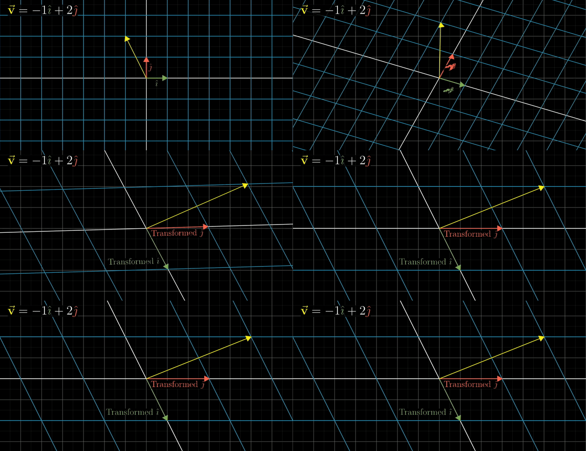
Although visually pretty, these animations can sometimes obscure our understanding.
In this post, we will distill a matrix transformation down to two processes: the “before” and “after”. In the before (pictured left), we will break the vector that is being transformed into its components along a basis. In the after (pictured right), we will move those components to a new basis, and then reconstruct the vector in that new basis. The full process is shown below with draggable sliders (to have them move automatically after dragging them, refresh the page).


Now that we understand the full process, there are really only two pictures we want to store in our brain:
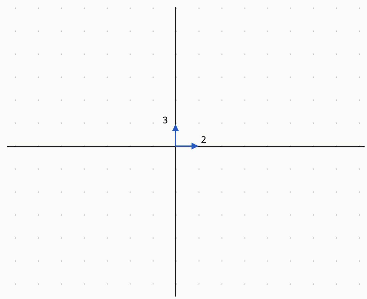
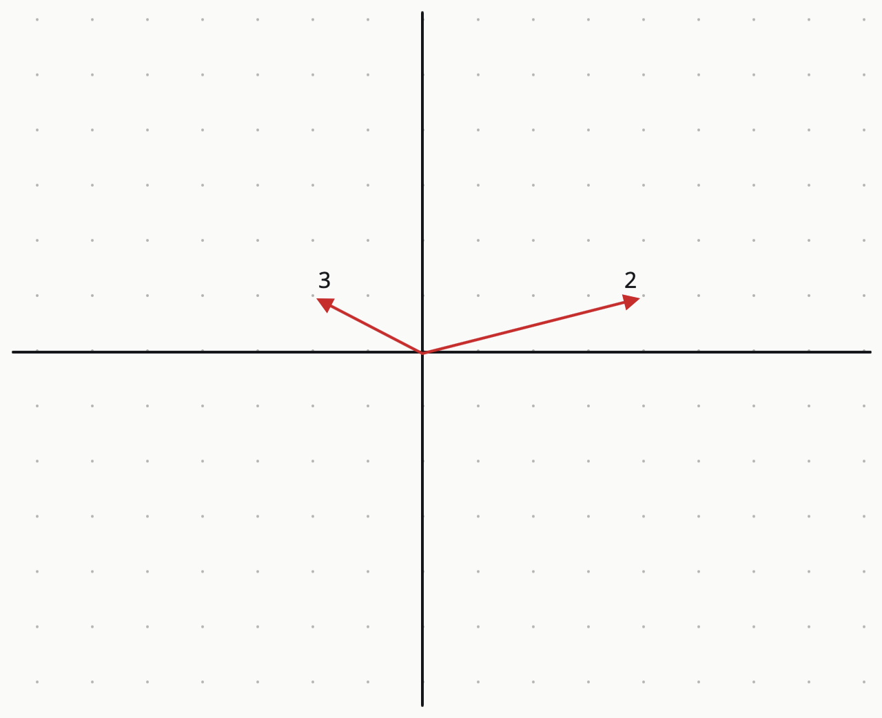
For the rest of this post, do not try to combine the resulting vectors into a final result. It will only muddy your understanding.
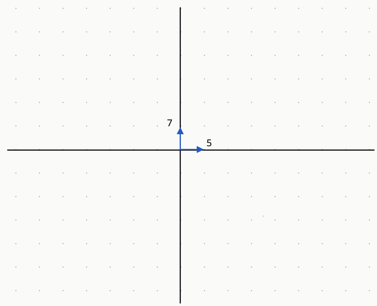
Let’s try to transform the vector \(x = \begin{bmatrix} 5 \\ 7 \end{bmatrix}\) by the same matrix \(A\) above. What are the two pictures we should store in our brain?

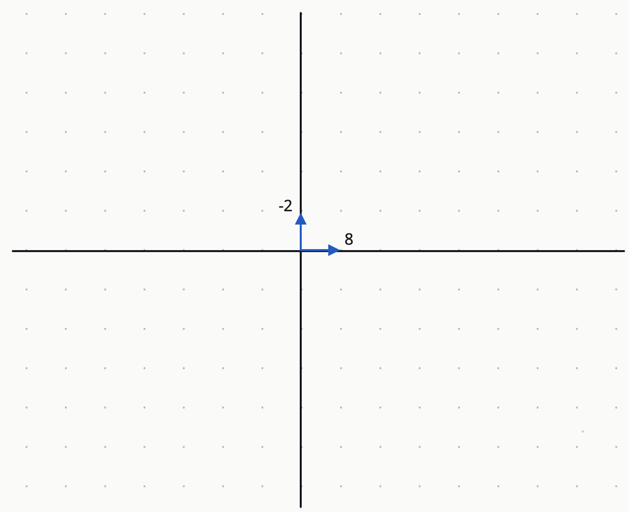
Great! Now let’s try to transform the vector \(x = \begin{bmatrix} 8 \\ -2 \end{bmatrix}\):
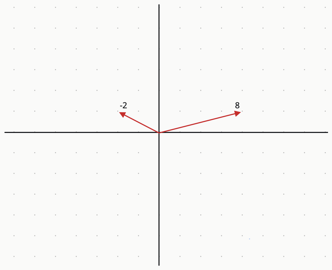
Nice, you’re a pro!
Now take a moment to reflect on this perspective. Why does this feel so easy?
Shortcomings
At the end of the day, it would be nice to know something useful about where the final vector will lie in space once the vectors and their associated components in the “after” snapshot are combined. This is hard to do, because the vectors in the “after” snapshot can be pointing any which way.
Crucially, this means that the red vectors interfere with each other, and we need to think about all of them at the same time to have a good visualization of where the final vector will end up.
It would be really nice if we could have the vectors in the “after” snapshot point in directions that were more intuitive to us and had less interference with one another. Thinking back to “Track the Point”, we may be looking at this linear transformation with the wrong basis.
That would make things much simpler.
What is an SVD
- Bertrand Russell
The red vectors in the “after” snapshot are the column vectors of \(A\). It would be nice if the column vectors of \(A\) were all orthogonal, but this might not be the case.
What the SVD says is that if we are okay rotating our blue basis vectors
It may seem strange that we’re allowed to do this. Soon, we’ll resolve these concerns.
Algebraic Definition
All matrices \(A \in R^{m \times n}\) can be written as \(A = U \Sigma V^T\) where \(U \in R^{m \times m}\) consists of \(m\) orthonormal vectors, \(V \in R^{n \times n}\) consists of \(n\) orthonormal vectors, and \(\Sigma \in R^{m \times n}\) is a diagonal matrix with non-negative elements along the diagonal and zeroes in all other entries. Written out, it looks like this
\[A = \begin{bmatrix} | & | & \dots & | \\ \vec{u_1} & \vec{u_2} & \dots & \vec{u_m} \\ | & | & \dots & | \\ \end{bmatrix} \begin{bmatrix} \sigma_1 & 0 & \dots & 0 \\ 0 & \sigma_2 & \dots & 0 \\ \vdots & \vdots & \ddots & \vdots \\ 0 & 0 & \dots & \sigma_{\min(m,n)} \\ \end{bmatrix} \begin{bmatrix} - & \vec{v_1}^T & - \\ - & \vec{v_2}^T & - \\ \vdots & \vdots & \vdots \\ - & \vec{v_n}^T & - \\ \end{bmatrix}\]where \(\sigma_1, \sigma_2, \dots, \sigma_n \geq 0\).
\(\Sigma\) is a weird shape, and we encourage the reader to not worry about the shape too much, just remember that it is a diagonal matrix with non-negative values on the diagonal. If this feels like complicated algebra soup, don’t worry. We will now go through what each of these matrices mean.
Geometric Visualization
For the rest of this post we will assume the above definition is correct and the SVD exists for all matrices (proof in appendix). Geometrically, how does the SVD \(A = U \Sigma V^T\) help us understand what happens to a vector when we multiply it by \(A\)?
\[\begin{align*} A x &= U \Sigma V^T x \\ &= (U \Sigma) (V^T x) \\ \end{align*}\]First, \(V^T x\) represents the components of \(x\) in the basis of \(V\), because \(V^T = V^{-1}\) (proof in appendix). You can think of it as \(V (V^T x)\) will recover \(x\) so \(V^T x\) must be the components of \(x\) in the basis of \(V\).
Next, the matrix \(U \Sigma\) represents orthogonal vectors. They are the orthonormal column vectors of \(U\) that have each been scaled by a non-negative factor in \(\Sigma\):
\[\begin{bmatrix} \\ \vec{u_1} & \vec{u_2} & \dots & \vec{u_m} \\ \\ \end{bmatrix} \begin{bmatrix} \sigma_1 & 0 & \dots & 0 \\ 0 & \sigma_2 & \dots & 0 \\ \vdots & \vdots & \ddots & \vdots \\ 0 & 0 & \dots & \sigma_{m} \\ \end{bmatrix} = \begin{bmatrix} \\ \sigma_1 \vec{u_1} & \sigma_2 \vec{u_2} & \dots & \sigma_{m} \vec{u_{m}} \\ \\ \end{bmatrix}\]So when we multiply \(U \Sigma\) by \(V^T x\), essentially what we are doing is for each \(v_i \in V\) we are taking the component of \(x\) in the \(\vec{v_i}\) direction (the “before” snapshot) and moving it to the \(\vec{u_i}\) direction (the “after” snapshot), while also scaling it by \(\sigma_i\). Feel free to reread this section again, because it is the most important part of this blogpost.
Before we transformed vectors like this:


But now we can transform vectors this way:


This is very exciting! If we choose to start by thinking about a vector in the correct basis (namely \(V\)), it’s very easy to see where it will end up after the transformation. If the component of \(\vec{x}\) in the \(\vec{v_i}\) direction is \(c_i\), then the component of \(A\vec{x}\) in the \(\vec{u_i}\) direction will be \(\sigma_i c_i\).
Now we can essentially discard the matrix \(A\), and whenever we want to understand what \(A\) does, we’ll just think of \(U\), \(\Sigma\), and \(V\) instead. For any starting vector \(x\), we look at it in terms of the \(V\) basis, scale the components, and place them along the respective \(U\) basis vectors. Once again, feel free to let this entire section sink in as it’s the most important part of the blogpost.
This geometric perspective is a very powerful idea, and we’ll see how it can be used in practice later in the post.
Rectangular Matrices
What happens when \(A \in \mathbb{R}^{m \times n}\) isn’t square? The SVD still exists and \(U \in \mathbb{R}^{m \times m}\), \(V \in \mathbb{R}^{n \times n}\), but there are two cases to consider:
If \(m > n\), then we will have orthonormal vectors \(u_1, \dots, u_n, u_{n+1}, \dots, u_m\) and \(v_1, \dots, v_n\), and the \(v_i\) component will be scaled by \(\sigma_i\), for all \(1 \leq i \leq n\). In addition, \(u_{n+1}, \dots, u_m\) will not be reachable, so their components after a transformation will always be zero. This projects up from an \(n\) dimensional space into a \(m\) dimensional space. While the resulting space exists in \(m\) dimensions, it will still be an \(n\) dimensional subspace.
If \(m < n\), then we will have orthonormal vectors \(u_1, \dots, u_m\) and \(v_1, \dots, v_m, v_{m+1}, \dots, v_{n}\), and the \(v_i\) component will be scaled by \(\sigma_i\), for all \(1 \leq i \leq m\). In addition, \(v_{m+1}, \dots, v_n\) will not map to any basis vectors of \(U\), so their components can be effectively ignored when thinking about the transformation (as they will be deleted).
If this section feels confusing, try to think about the before and after picture. If there’s more vectors in the after picture, there will be no vectors in the before picture to map to them, so their components will be 0 (\(m > n\)). If there’s more vectors in the before picture, there’s no vectors in the after picture for them to map to, so their components will not be used (\(m < n\)).
Computing \(U\), \(\Sigma\), \(V\) in Practice
Conveniently, we have
\[\begin{align} A^T A &= (V \Sigma U^T) (U \Sigma V^T) \\ &= (V \Sigma) (U^T U) (\Sigma V^T) \\ &= (V \Sigma) (\Sigma V^T) \\ &= V \Sigma^2 V^T \end{align}\](1) follows from the formula for a transpose (proof), (2) follows from matrix multiplication being associative, and (3) follows from \(U\) being an orthonormal matrix (proof in appendix). From (4), one can compute \(V\) and \(\Sigma\) by finding an eigendecomposition of \(A^T A\).
Similarly, \(A A^T = U \Sigma^2 U^T\), so we can compute \(U\) and \(\Sigma\) by taking the eigenvectors and eigenvalues of \(A A^T\). The topic of solving for eigenvectors is beyond the scope and value of this post, though a curious reader can find resources online. The key idea to take away is that you can indeed compute \(U\), \(\Sigma\), and \(V\) in practice if you need to.
Why is this useful?
- Richard Hamming
Qualitatively, we should make a few comments about the SVD:
- No matter what matrix we’re working with, the SVD always exists, and it’s basically unique.
- The SVD is actually what the matrix “is.” It’s a completely equivalent (and more helpful) way to think about the transformation.
A good trick I’ve found when encountering situations in linear algebra (even ones with dense matrix algebra that can be hard to follow) is to start by writing matrices in terms of their SVD. Oftentimes, everything starts to quickly make sense. Let’s go through a few examples together of where this approach was personally helpful for me.
Transpose of a Matrix
We’ve all heard of the transpose of a matrix \(A^T\).
At first we might guess it’s the inverse. While this is true for orthonomal matrices (proof in appendix), it is not in general. This can be quite baffling, what actually is \(A^T\)? We might try reasoning from a smaller matrix we can more easily wrap our heads around:
\[A = \begin{bmatrix} a_{11} & a_{12} & a_{13} \\ a_{21} & a_{22} & a_{23} \\ a_{31} & a_{32} & a_{33} \end{bmatrix}, \text{ so } A^T = \begin{bmatrix} a_{11} & a_{21} & a_{31} \\ a_{12} & a_{22} & a_{32} \\ a_{13} & a_{23} & a_{33} \end{bmatrix}\]So with \(A\) we map the unit vector \(\begin{bmatrix} 1 \\ 0 \\ 0\end{bmatrix}\) to \(\begin{bmatrix} a_{11} \\ a_{21} \\ a_{31}\end{bmatrix}\) but with \(A^T\) we map it to \(\begin{bmatrix} a_{11} \\ a_{12} \\ a_{13}\end{bmatrix}\). Hmm, that still seems weird and doesn’t give us any insight.
What if we start by writing it in terms of its SVD? We have \(A = U \Sigma V^T\), and \(A^T = V \Sigma U^T\). Let’s try to visually understand what \(A\) is doing in space.
\(A\) starts with the basis \(V\), and stretches it by the singular values \(\Sigma\), and then rotates it to the basis \(U\). Wait a second… based on the equation for \(A^T\) (which is also the SVD of \(A^T\)) \(A^T\) starts with the basis \(U\), and stretches it by the singular values \(\Sigma\), and then rotates it to the basis \(V.\) Woah! Now we can picture what \(A^T\) does to space relative to \(A\).
So it seems that \(A^T\) is kind of like an inverse of \(A\) in that \(A\) switches the basis from \(V\) to \(U\), and \(A^T\) switches it back from \(U\) to \(V\). But it’s not entirely so, because rather than undoing the singular value scaling on each of the components from \(A\), it applies the same scaling again to each of the components from \(A\). So after transforming by \(A\) and then \(A^T\) the thing we should get are the same components in the \(V\) basis, but scaled by the singular values twice, which would be \(V \Sigma^2 V^T\) (remember, \(V^T\) means write components in terms of the \(V\) basis, \(\Sigma^2\) means scale them twice by \(\Sigma\), and \(V\) means construct the vector from the perspective of the \(V\) basis with each of those components)… Woah, that’s what we get when we multiply \(A^T A\).
Kind of cool that we now understand this commonplace concept. This is only the beginning of what we can do with SVD.
Dot Product Preservation
You may have seen before that \(Ax \cdot Ay = x \cdot A^T A y\). Using properties of transposes, we could prove this fairly quickly:
\[\begin{align*} Ax \cdot Ay &= (Ax)^T(Ay) \\ &= (x^T A^T) (A y) \\ &= x^T A^T A y \\ &= x^T (A^T A y) \\ &= x \cdot (A^T A y) \end{align*}\]But writing off this property to algebraic operations would be missing a beautiful geometric interpretation and internalization of the concept. Isn’t it crazy that if you want to know what the dot product of \(x\) and \(y\) will be after a matrix transformation, you don’t need to transform them both? You only need to transform one of them by a different matrix (\(A^T A\) in this case) and then dotting from there will get the desired answer? It’s totally wild that \(A^T A\) will transform \(y\) so that the length of \(A^T A y\) and the angle between \(A^T A y\) and \(x\) is exactly what it needs to be to match the lengths of \(Ax\), \(Ay\), and the angle between them.
How could this be? When exploring this question without our SVD enlightenement, this phenomena feels hazy. But with our new perspective, perhaps we can distill the insight. Since the SVD seems to be changing basis often, as we reason through this we should keep in mind that the dot product between two vectors is constant regardless of what basis we use to compute it.
We can start by thinking about what the dot product of \(x\) and \(y\) looks like from the perspective of \(A\)’s SVD. The SVD of \(A\) wants to start by thinking about the components of \(x\) and \(y\) in the \(V\) basis, so that’s what we do. Conveniently, we can think about the dot product in the basis of \(V\) since it stays the same across any basis. Then, \(Ax\) and \(Ay\) each have the same components dotted with each other as before, but they are now situated along the \(U\) basis and are each scaled by a \(\sigma\). So if \(c_{ix}\) denotes the component of \(x\) along \(v_i\) and similarly for \(c_{iy}\), then
\[\begin{align*} x \cdot y &= \sum_{i=1}^n c_{ix} c_{iy} \\ Ax \cdot Ay &= \sum_{i=1}^n (\sigma_i c_{ix}) (\sigma_i c_{iy}) \end{align*}\]Now let’s think about what \(A^T A\) does visually. It scales the components in the \(V\) direction by \(\sigma\) twice, but keeps those components situated along \(V\) because \(A\) moves from the \(V\) basis to the \(U\) basis, and then \(A^T\) moves from the \(U\) basis back to the \(V\) basis. This means
\[\begin{align*} x \cdot A^T Ay &= \sum_{i=1}^n (c_{ix}) (\sigma_i^2 c_{iy}) \end{align*}\]so clearly \(x \cdot A^T Ay = Ax \cdot Ay\), but now we can see why this happens visually, giving us more insight into why the property is true. It’s not that the angle between \(x\) and \(A^T A y\) is the same as the angle between \(Ax\) and \(Ay\), nor is it true that the product of their magnitudes is equivalent: \(\| x \| \| A^T Ay \| = \| Ax \| \| Ay \|\). Rather, this \(x \cdot A^T Ay = Ax \cdot Ay\) property holds because when we think about the transformations from the perspective of the right basis, we see that instead of scaling the \(i^{th}\) coordinate by \(\sigma_i\) in both \(x\) and \(y\), we scale it by \(1\) in \(x\) and \(\sigma_i^2\) in \(y\), keeping the dot product unchanged.
Although algebra is written above to be more precise, the reader is highly encouraged to try visualizing this phenomena.
Linear Regression
After internalizing the geometric perspective presented earlier in this post, I was able to reason through linear regression when I encountered it in a paper about Demystifying Double Descent,
In linear regression, we want to find the vector \(x\) that minimizes the distance between \(Ax\) and \(b\). Mathematically, for \(A \in \mathbb{R}^{m \times n}\) and \(b \in \mathbb{R}^m\), we want to find the \(x \in \mathbb{R}^n\) that minimizes \(\| Ax - b \| _2^2\). Typically \(m > n\) which means we have a system of \(m\) equations in \(n\) variables, so we can’t get a perfect solution.
The solution to this problem turns out to be \(x = (A^T A)^{-1} A^T b\). Where did all these weird symbols, transposes, and inverses come from?
If you look up proofs for this formula, you’ll find they often use matrix calculus and are very symbol heavy. Whenever something in linear algebra seems complicated, we start from the beginning with the SVD and try reasoning about what’s going on.
Replacing \(A\) with \(U \Sigma V^T\) we want to find an \(x\) that after scaling by \(\Sigma\) in the \(V\) directions, and moving the components to the \(U\) basis, gets us as close to \(b\) as possible.
Because \(m > n\), we will have more \(U\) basis directions than \(V\) basis directions. This means that some of our \(U\) basis directions are not reachable by any vector in the \(V\) subspace (i.e. they don’t have a corresponding basis vector in \(V\)).
But for the basis directions of \(U\) that are reachable, we will want those components to be exactly equal to the components of \(b\) in the \(U\) basis to minimize the norm of \(Ax-b\). So the thing we want to do is take the vector \(b\), write it in terms of it’s \(U\) directions, scale it by \(\frac{1}{\sigma_i}\) if that direction is reachable and 0 otherwise. Then rotate those resulting components to the \(V\) basis which reconstructs the optimal \(x\). In terms of matrices, this looks like:
\[\begin{align*} x &= \underbrace{\begin{bmatrix} \\ \vec{v_1} & \vec{v_2} & \dots & \vec{v_n} \\ \\ \end{bmatrix} \overbrace{\begin{bmatrix} \sigma_1^{-1} & 0 & \dots & 0 \\ 0 & \sigma_2^{-1} & \dots & 0 \\ \vdots & \vdots & \ddots & \vdots \\ 0 & 0 & \dots & \sigma_{n}^{-1} \\ \end{bmatrix} \underbrace{\begin{bmatrix} & & & \vec{u_1} & & & \\ & & & \vec{u_2} & & & \\ & & & \vdots & & & \\ & & & \vec{u_m} & & & \end{bmatrix} b}_{\text{This writes } b \text{ in the } U \text{ basis}}}^{\text{Components of } b \text{ in the } U \text{ basis scaled by the appropriate } \sigma \text{ values}}}_{\text{Components of } b \text{ in the } U \text{ basis scaled by the appropriate } \sigma \text{ values and moved to the } V \text{ basis}} \\ &= V \Sigma^{-1} U^T b. \end{align*}\]When we write \(\Sigma^{-1}\), we mean the matrix where we take the reciprocal of each of the diagonal entries, while leaving the ones that are zero as zero.
Our answer doesn’t quite look like \(x = (A^T A)^{-1} A^T b\). Let’s see what happens when we substitute \(A = U \Sigma V^T\) and simplify (with lots of terms cancelling):
\[\begin{align*} (A^T A)^{-1} A^T b &= (V \Sigma U^T U \Sigma V^T)^{-1} V \Sigma U^T b \\ &= (V \Sigma \Sigma V^T)^{-1} V \Sigma U^T b \\ &= (V \Sigma^2 V^T)^{-1} V \Sigma U^T b \\ &= (V \Sigma^{-2} V^T) V \Sigma U^T b \\ &= V \Sigma^{-2} \Sigma U^T b \\ &= V \Sigma^{-1} U^T b \\ \end{align*}\]So we do get the same thing! Hopefully you are beginning to appreciate the beauty of reasoning through problems with the SVD. It’s amazing that we can actually visualize what’s happening!
There is a less known variant of the linear regression problem where we have \(m < n\) and want to minimize \(\| Ax - b \| _2^2\). Since we now have less equations than variables, there are typically many such solutions to this problem that perfectly optimize it, so the goal is to find the solution among the perfectly optimal ones such that \(\|x\| _2^2\) is minimized.
This feels even trickier than the previous problem. It’s not even immediately clear where to begin if we were to use matrix calculus. The solution to this problem turns out to be \(x = A^T (A A^T)^{-1} b\), another weird combination of symbols, transposes, and inverses. Let’s see if we can understand this on our own with SVD.
Replacing \(A\) with \(U \Sigma V^T\) we want to find an \(x\) that after scaling by \(\Sigma\) in the \(V\) directions, and moving the components to the \(U\) basis, gets us exactly \(b\) (or at least as close as possible).
Because \(m < n\), we will have more \(V\) basis directions than \(U\) basis directions. This means that some of our \(V\) basis directions have no effect on the final vector in the \(U\) subspace.
But for the basis directions of \(V\) that do have corresponding basis vectors in \(U\), we will want those components (after transformation) to be exactly equal to the components of \(b\) in the \(U\) basis to minimize the norm of \(Ax-b\). So the thing we want to do is take the vector \(b\), write it in terms of it’s \(U\) directions, and scale those by \(\frac{1}{\sigma_i}\) to get the components in our corresponding \(V\) directions.
It’s quite interesting that for both variants where \(m>n\) and \(m<n\), the solution to the problem is precisely \(V \Sigma^{-1} U^T\). Substituting this into \(x = A^T (A A^T)^{-1} b\) we get
\[\begin{align*} A^T (A A^T)^{-1} b &= V \Sigma U^T (U \Sigma V^T V \Sigma U^T)^{-1} b \\ &= V \Sigma U^T (U \Sigma \Sigma U^T)^{-1} b \\ &= V \Sigma U^T (U \Sigma^2 U^T)^{-1} b \\ &= V \Sigma U^T (U \Sigma^{-2} U^T) b \\ &= V \Sigma \Sigma^{-2} U^T b \\ &= V \Sigma^{-1} U^T b \\ \end{align*}\]So we indeed get our answer.
If both these answers are “the same”, then why is one written like \((A^T A)^{-1} A^T\) and the other written like \(A^T (A A^T)^{-1}\)? The key idea is that to compute \(\Sigma^{-1}\) in terms of the original matrix \(A\), we need to take an “inverse” somehow, and we can simply invert \(A^T A\) or \(A A^T\) since they are both square matrices. The distinction comes in because when \(m>n\) only \(A^T A\) is invertible, and when \(m<n\) only \(A A^T\) is invertible.
Considering that our answer (written in terms of the SVD) is intuitive and holds for both problem formulations, perhaps SVD is fundamentally the core way to think about the concept of linear regression. 🙂
Conclusion
Matrices are the fundamental building blocks of machine learning, and we have found a useful way to understand them through their SVD. When we select the right starting and ending basis for a matrix transformation, we can think of each component independently of the others, giving us a clear picture of everything going on in the transformation.
Not only is the SVD theoretically beautiful, but it’s also incredibly practical for clarifying complicated matrix concepts we encounter in our work. The SVD often singlehandedly distills matrix algebra to crisp, intuitive explanations of underlying phenomena. This suggests that the SVD not only exists for all matrices, but that the rotations and scalings present in SVD are the true units of computation we should be considering when working with matrices.
Hence, the SVD is an incredibly powerful tool for understanding matrices. When you encounter matrices in the future, we hope you find success in reasoning about them through the SVD.
Acknowledgements
Special thanks to [insert names here] and how they helped, to be added after rounds of feedback are received.
I would also like to thank the authors of the resources listed below, without whom my understanding of matrices would not be as strong.
Written Resources
- Six (and a half) intuitions for SVD by Callum McDougall
- Lecture 4. The Singular Value Decomposition by Cornell CS 322
- Singular Value Decomposition as Simply as Possible by Gregory Gundersen
- What is an intuitive explanation of singular value decomposition (SVD)? by Quora users
Video Resources
- Linear Algebra video series by 3Blue1Brown
- What is the Singular Value Decomposition? by Stochastic
- SVD Visualized, Singular Value Decomposition explained by Visual Kernel
Appendix
Inverse of Orthonormal Matrix
A key property of orthonormal matrices is that its transpose is its inverse. Specifically for an orthonormal matrix \(Q\):
\[Q^T Q = \begin{bmatrix} - & \vec{q_1}^T &- \\ - & \vec{q_2}^T &- \\ \vdots & \vdots & \vdots \\ - & \vec{q_n}^T &- \end{bmatrix} \begin{bmatrix} | & | & \dots & | \\ \vec{q_1} & \vec{q_2} & \dots & \vec{q_n} \\ | & | & \dots & | \end{bmatrix} = \begin{bmatrix} 1 & 0 & \dots & 0 \\ 0 & 1 & \dots & 0 \\ \vdots & \vdots & \ddots & \vdots \\ 0 & 0 & \dots & 1 \\ \end{bmatrix}\]This is due to the orthonormality condition, where \(q_i^T q_j = 0\) if \(i \neq j\) and \(q_i^T q_j = 1\) if \(i = j\).
SVD Existence Proof
Here we’ll walk through an intuitive proof to convince us that the SVD in fact exists for any matrix \(A\).
Singular values seem to scale matrices in independent directions by varying amounts. So we begin by considering the unit vector that has the greatest norm after being transformed by \(A\), i.e. the vector that \(A\) stretches the most. We will call this vector \(v_1\), and the vector it gets mapped to \(\sigma_1 u_1\) where \(\|u_1\| = 1\):
\[\begin{align*} v_1 &= \underset{\|x\| = 1}{\mathrm{argmax}} \|Ax\| \\ Av_1 &= \sigma_1 u_1 \end{align*}\]If it was true that for all unit vectors \(v_2\) orthonormal to \(v_1\), \((Av_2) \cdot u_1 = 0\), then we would have that \(v_1\) is the only starting vector that has any component in the \(u_1\) direction after being mapped by \(A\). We could then pick a \(v_2\) orthonormal to \(v_1\) such that it maximally stretches the remaining subspace with zero component in the \(v_1\) direction. We would also have \(Av_2 = \sigma_2 u_2\) orthogonal to \(u_1\) because \(v_2\) is orthonormal to \(v_1\). We could continue doing this by induction until the entire input space is spanned, which shows that SVD exists.
So now the only thing we have left to do is show that in fact:
\[\begin{equation*} v_2 \cdot v_1 = 0 \implies Av_2 \cdot u_1 = 0 \quad \forall v_2 \end{equation*}\]Suppose this was false, and that there was some vector \(v_2\) (orthogonal to \(v_1\)) such that \(Av_2\) has a component \(\epsilon > 0\) in the \(u_1\) direction (if the component is negative we use \(-v_2\) instead which will have a positive component).
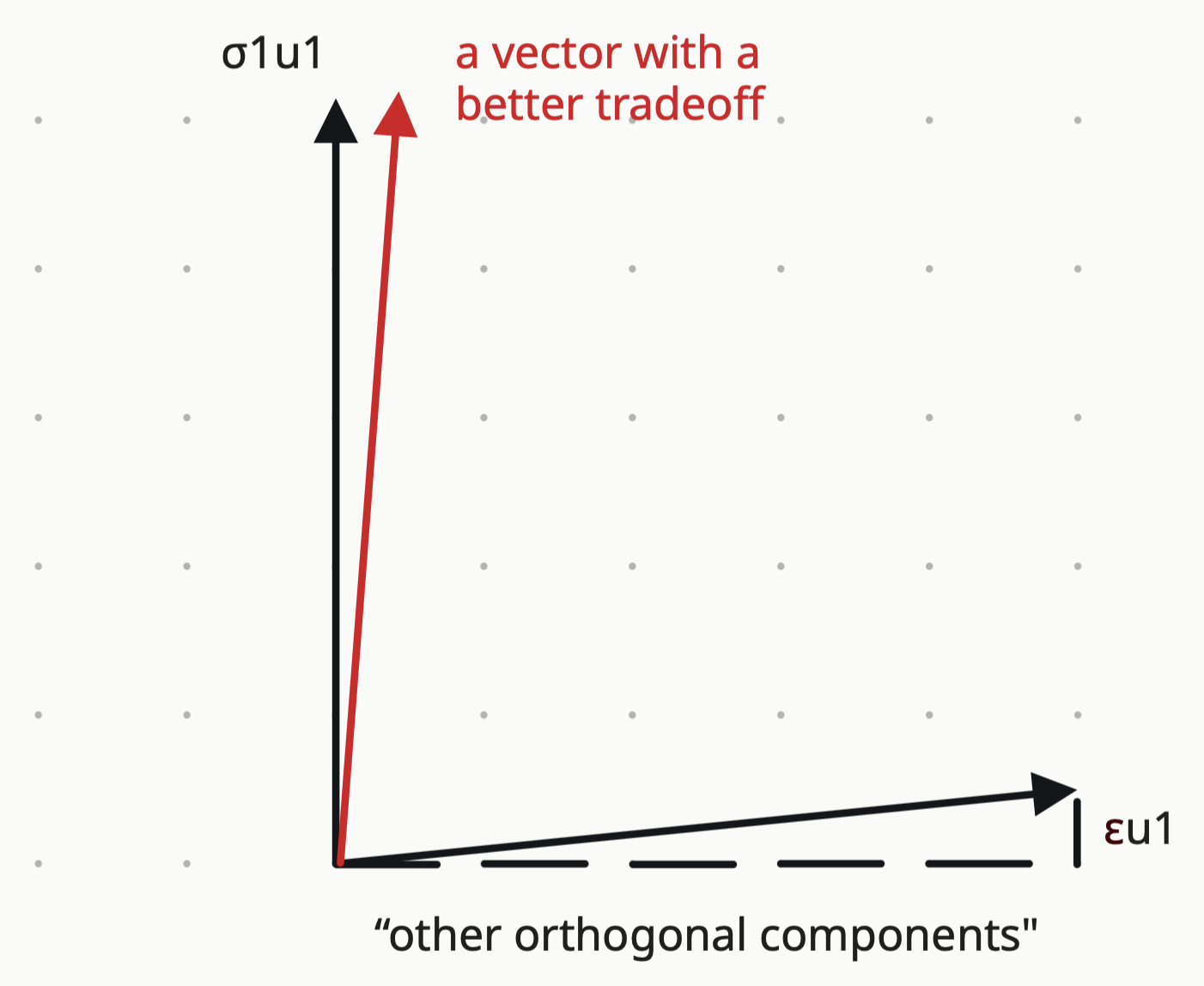
Now, let’s think about the set of unit vectors \(\alpha v_1 + \beta v_2\) where \(\alpha, \beta \in \mathbb{R}\) are constants and \(\alpha^2 + \beta^2 = 1\). When \(\alpha = 0, \beta = 1\) we get \(v_2\), when \(\alpha = 1, \beta = 0\) we get \(v_1\). When we have \(\alpha = 1, \beta = 0\), if we nudge \(\alpha\) down a tiny-bit, say by \(\delta\), then \(\beta\) will shoot up to \(\sqrt{2 \delta - \delta^2}\).
However, since \(\sigma_1\) and \(\epsilon\) are just constants, it is certainly true that for small enough \(\delta\):
\[\underbrace{\sigma_1 \delta}_{\text{component we lose in } u_1 \text{ direction by moving away from } v_1} < \underbrace{\epsilon \sqrt{2 \delta - \delta^2}}_{\text{component we gain by nudging } v_1 \text{ toward } v_2}\]Hence, our tradeoff near \(v_1\) says it is much better for us to nudge \(v_1\) toward \(v_2\) to maximize the component in the \(u_1\) direction.
This means that \(v_1 \neq \underset{\|x\| = 1}{\mathrm{argmax}} \|Ax\|\), which is a contradiction. Hence, our assumption was false, and we have that \(v_2 \cdot v_1 = 0 \implies Av_2 \cdot u_1 = 0 \quad \forall v_2\), finishing the proof.
If this section about SVD existence was not crystal clear, it’s fine to move past it. The geometric visualization is by far the most important section to internalize from this post.